3D partitioned heat conduction

We solve a simple heat equation on a 3D domain. The domain is partitioned and the coupling is established in a Dirichlet-Neumann fashion.

Note: Get the case files of this tutorial, as continuously rendered here, or see the latest released version (if there is already one). Read how in the tutorials introduction.

Setup

We solve a partitioned heat equation. For information on the two dimensional non-partitioned case, please refer to [1, p.37ff]. In this tutorial the computational domain is partitioned and coupled via preCICE. The coupling roughly follows the approach described in [2].

Case setup of partitioned-heat-conduction case

The computational domain can be seen in the picture above. To get a better overview of the domain, the domains of the participants are translated. The domain of the Neumann participant is the small box, and the Dirichlet participant’s domain is the rest. In the simulation, the small box is fully contained in the Dirichlet domain. This means, the coupling interface consists of five sides of the box.

Configuration

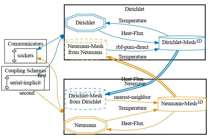
preCICE configuration (image generated using the precice-config-visualizer):

preCICE configuration visualization

Available solvers and dependencies

You can either couple a solver with itself or different solvers with each other. In any case you will need to have preCICE and the python bindings installed on your system.

FEniCSx. Install FEniCS and the FEniCSx-adapter. The code is adapted from the existing fenics-tutorial from [1].

Running the simulation

You can find the corresponding run.sh script for running the case in the folders corresponding to the participant you want to use:

cd dirichlet-fenicsx
./run.sh

and

cd neumann-fenicsx
./run.sh

Visualization

Output is written into the folders of the FEniCSx solvers (neumann-fenicsx/output-neumann.bp and dirichlet-fenicsx/output-dirichlet.bp).

It is sufficient to import the folders to ParaView to get the visualization of the simulation.

References

[1] Hans Petter Langtangen and Anders Logg. “Solving PDEs in Minutes-The FEniCS Tutorial Volume I.” (2016). pdf