Partitioned Burgers' equation 1D
Setup
We solve the 1D viscous Burgers’ equation on the domain \([0,2]\):
\[\frac{\partial u}{\partial t} = \nu \frac{\partial^2 u}{\partial x^2} - u \frac{\partial u}{\partial x},\]where \(u(x,t)\) is the scalar velocity field and \(\nu\) is the viscosity. In this tutorial by default \(\nu\) is very small (\(10^{-12}\)), but can be changed in the solver.
The domain is partitioned into participants at \(x=1\):
- Dirichlet: Solves the left half \([0,1]\) and receives Dirichlet boundary conditions at the interface.
- Neumann: Solves the right half \([1,2]\) and receives Neumann boundary conditions at the interface.
Both outer boundaries use zero-gradient conditions \(\frac{\partial u}{\partial x} = 0\). The problem can be solved for different initial conditions of superimposed sine waves, which can be generated using the provided script utils/generate_ic.py.
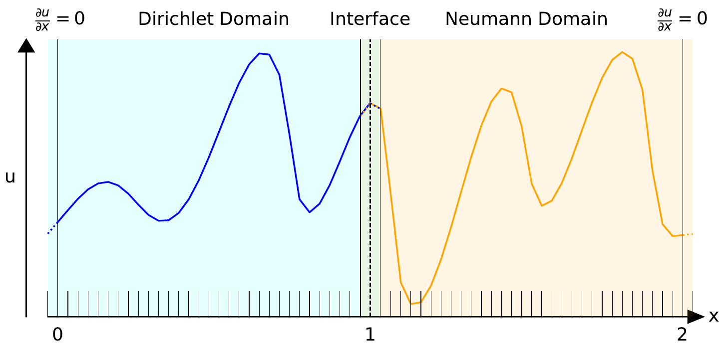 Diagram of the partitioned domain with an example initial condition.
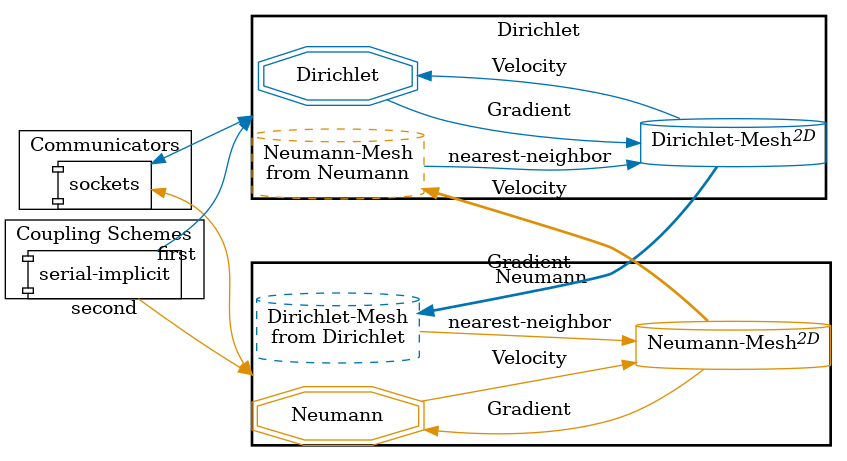
Configuration
preCICE configuration (image generated using the precice-config-visualizer):
Available solvers
Currently, the SciPy solver (solver-scipy) can be used for both sides, the NN surrogate solver (neumann-surrogate) only for the Neumann side.
- SciPy. Simple finite volume solver using Lax-Friedrichs fluxes and implicit Euler time stepping.
- Surrogate. Pre-trained neural network surrogate model.
The conservative formulation of the Burgers’ equation is implemented in the SciPy solver. The surrogate is a neural network trained to autoregressively predict the next time step solution based on the current solution. The surrogate model was trained on solutions obtained with the SciPy solver. See Initial condition for how to generate the training data.
Two pre-trained model checkpoints are provided in neumann-surrogate/, differing in how many unroll timesteps were used during the Backpropagation Through Time (BPTT) training phase. The two checkpoints, CNN_RES_UNROLL_1.pth and CNN_RES_UNROLL_7.pth, were trained, respectively, with a single-step prediction (rollout length 1) and a 7-step rollout, which improves stability over long autoregressive predictions. The checkpoint can be selected by changing MODEL_NAME in neumann-surrogate/config.py.
The full training pipeline [1] is available in a separate repository.
neumann-surrogate/requirements.txt. The GPU version requires several gigabytes of disk space (~6.2Gb).
Running the simulation
Running the participants
To run the partitioned simulation, open two separate terminals and start each participant individually:
You can find the corresponding run.sh script for running the case in the folders corresponding to the participant you want to use:
cd dirichlet-scipy
./run.sh
and
cd neumann-scipy
./run.sh
or, to use the pretrained neural network surrogate participant:
cd neumann-surrogate
./run.sh
Initial condition
The initial condition file initial_condition.npz is automatically generated by the run scripts if it does not exist.
You can also manually generate it using the utils/generate_ic.py script:
python3 utils/generate_ic.py
This script requires the Python libraries numpy and matplotlib. It accepts an optional argument --epoch as a random number generator seed, which defaults to zero.
To generate the training data, you can use the utils/generate-training-data.sh script from the tutorial root directory, which will generate data for different --epoch values:
./utils/generate-training-data.sh
Monolithic solution (reference)
You can run the whole domain using the monolithic solver for comparison:
cd solver-scipy
./run.sh
Post-processing
After both participants have finished, you can run the visualization script.
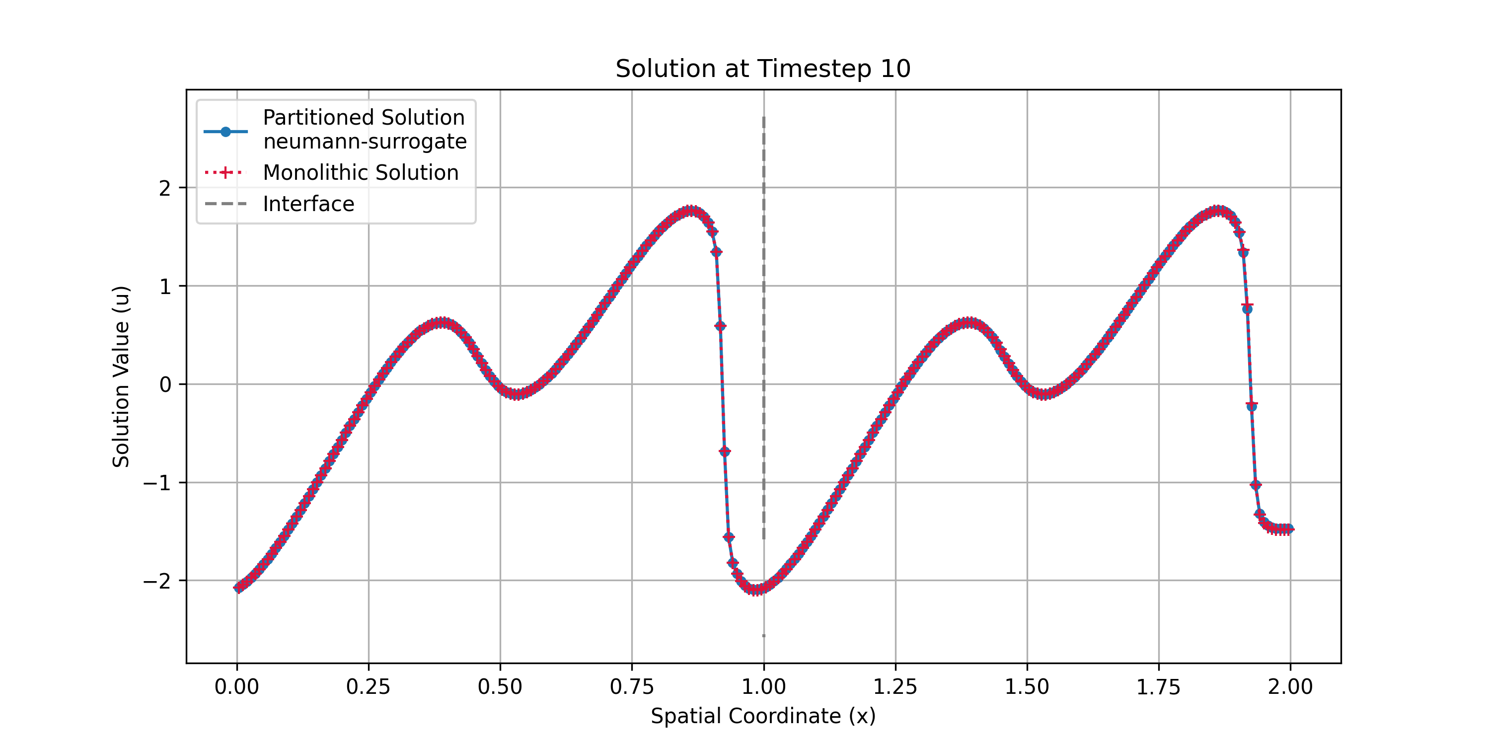
visualize_partitioned_domain.py generates plots comparing the partitioned and monolithic solutions. You can specify which timestep to plot. Call from the root of the tutorial:
python3 utils/visualize_partitioned_domain.py --neumann neumann-surrogate/surrogate.npz 10
The final argument defines the coupling time step to plot (here, 10). It can range from 0 up to the total number of time steps performed in the run.
The script will produce the following output files in the output/ directory:
full-domain-timestep-slice.png: Solution \(u\) at the selected timestep
-
gradient-timestep-slice.png: Gradient \(du/dx\) at the selected timestep -
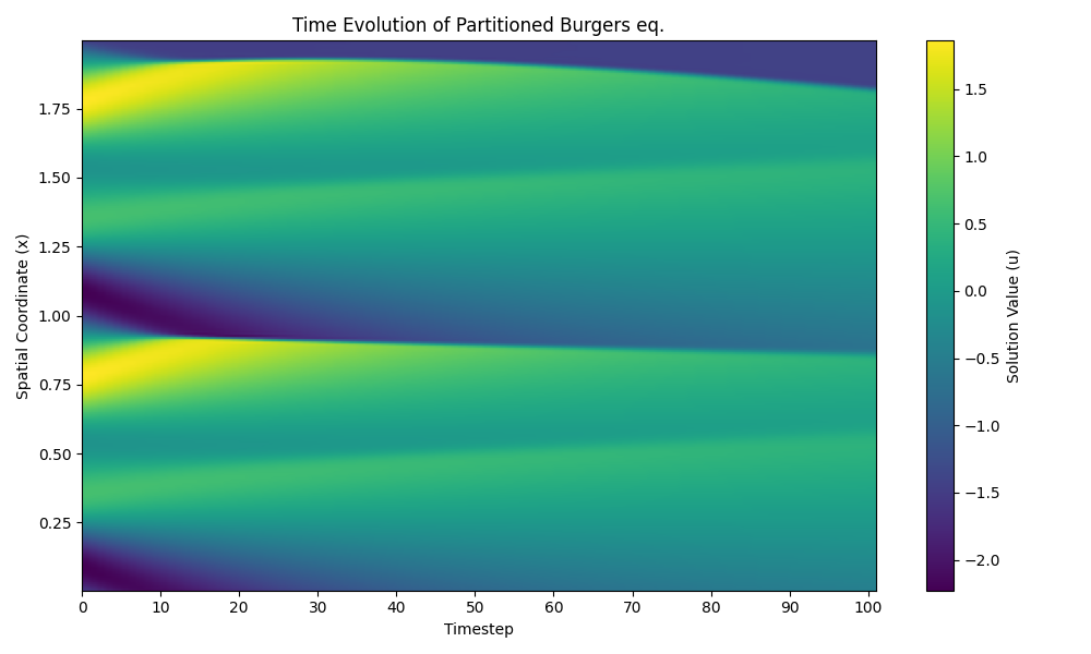
full-domain-evolution.png: Time evolution of the solution
References
[1] Dagis Daniels Vidulejs. “Coupling Neural Surrogates with Traditional Solvers using preCICE.” Master’s thesis, Technical University of Munich, 2025.