1D Elastic Tube
Setup
We want to simulate the internal flow in a flexible tube as shown in the figure below (image from [1]).
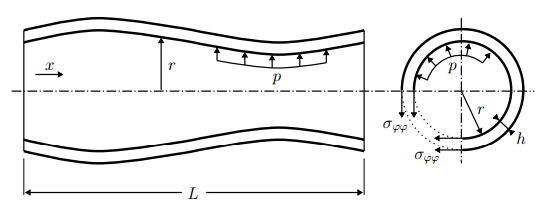
The flow is assumed to be incompressible flow and gravity is neglected. Due to the axisymmetry, the flow can be described using a quasi-two-dimensional continuity and momentum equations. The motivation and exact formulation of the equations that we consider can be found in [2].
The following parameters have been chosen:
- Length of the tube: L = 10
- Inlet velocity: \(v_{inlet} = 10 + 3 sin (10 \pi t)\)
- Initial cross sectional area = 1
- Initial velocity: v = 10
- Initial pressure: p = 0
- Fluid density: \(\rho = 1\)
- Young modulus: E = 10000
Additionally the solvers use the parameters N = 100 (number of cells), tau = 0.01 (dimensionless timestep size), kappa = 100 (dimensionless structural stiffness) by default. These values can be modified directly in each solver.
Configuration
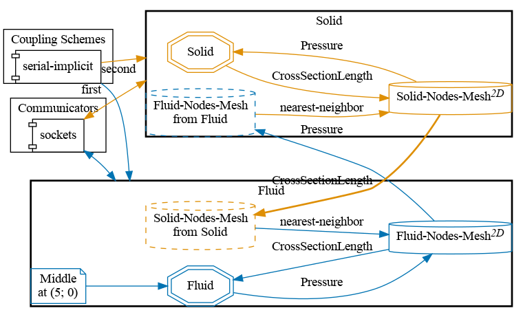
preCICE configuration (image generated using the precice-config-visualizer):
Available solvers
Both fluid and solid participant are supported in:
- C++: example solvers using the intrinsic C++ API of preCICE. The fluid solver also depends on LAPACK (e.g. on Ubuntu
sudo apt-get install liblapack-dev) - Python: example solvers using the preCICE Python bindings. The run script installs these automatically via pip in a virtual environment.
- Rust: example solvers using the preCICE Rust bindings. They need
cargoto be installed.
Running the Simulation
Choose one solver for each participant, then open two separate terminals and start each solver by calling the respective run script. Here we use both C++ solvers:
cd fluid-cpp
./run.sh
and
cd solid-cpp
./run.sh
Optional for python-fluid: A run-time plot visualization can be triggered by passing --enable-plot in run.sh of FluidSolver.py. Additionally a video of the run-time plot visualization can be generated by additionally passing --write-video
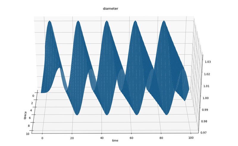
Post-processing
The results from each simulation are stored in each fluid-<participant>/output/ folder. You can visualize these VTK files using the provided plot-diameter.sh script
./plot-diameter.sh
which will try to visualize the results from both fluid cases, if available. This script calls the more flexible plot-vtk.py Python script, which you can use as
python3 plot-vtk.py <quantity> <case>/output/<prefix>
Note the required arguments specifying which quantity to plot (pressure, velocity or diameter) and the name prefix of the target vtk files.
For example, to plot the diameter of the fluid-python case using the default prefix for VTK files, plot-diameter.sh executes:
python3 plot-vtk.py diameter fluid-python/output/out_fluid_
Comparing different Fluid results
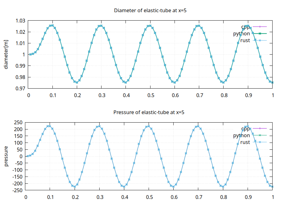
The Fluid participant defines a watchpoint at x=5, which records pressure and diameter for every timestep.
To compare the results of the various Fluid participants, you can run them all and plot the watchpoints using plot-all.sh.
The following is an example of running all Fluid solvers against the solid-cpp solver:
References
[1] B. Gatzhammer. Efficient and Flexible Partitioned Simulation of Fluid-Structure Interactions. Technische Universitaet Muenchen, Fakultaet fuer Informatik, 2014.
[2] J. Degroote, P. Bruggeman, R. Haelterman, and J. Vierendeels. Stability of a coupling technique for partitioned solvers in FSI applications. Computers & Structures, 2008.
[3] M. Mehl, B. Uekermann, H. Bijl, D. Blom, B. Gatzhammer, and A. van Zuijlen. Parallel coupling numerics for partitioned fluid-structure interaction simulations. CAMWA, 2016.