Oscillator

Setup

This tutorial solves a simple mass-spring oscillator with two masses and three springs. The system is cut at the middle spring and solved in a partitioned fashion:

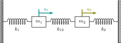
Note that this case applies a Schwarz-type coupling method and not (like most other tutorials in this repository) a Dirichlet-Neumann coupling. This results in a symmetric setup of the solvers. We will refer to the solver computing the trajectory of $m_1$ as Mass-Left and to the solver computing the trajectory of $m_2$ as Mass-Right. For more information, please refer to [1].

Configuration

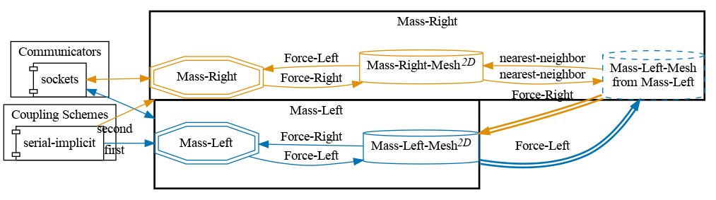
preCICE configuration (image generated using the precice-config-visualizer):

Available solvers

There are two different implementations:

• Python: A solver using the preCICE Python bindings. This solver also depends on the Python libraries numpy, which you can get from your system package manager or with pip3 install --user <package>. Using the option -ts allows you to pick the time stepping scheme being used. Available choices are Newmark beta, generalized alpha, explicit Runge Kutta 4, and implicit RadauIIA. The solver uses subcycling: Each participant performs 4 time steps in each time window. The data of these 4 substeps is then used by preCICE to create a third order B-spline interpolation (waveform-degree="3" in precice-config.xml).
• FMI: A solver using the preCICE-FMI runner (requires at least v0.2). The Runner executes the FMU model Oscillator.fmu for computation. The provided run scripts (see below) build this model if not already there. For more information, please refer to [2].

Running the simulation

Open two separate terminals and start both participants. For example, you can run a simulation where the left participant is computed in Python and the right participant is computed with FMI with these commands:

cd mass-left-python
./run.sh

and

cd mass-right-fmi
./run.sh

Of course, you can also use the same solver for both sides.

Post-processing

Each simulation run creates two files containing position and velocity of the two masses over time. These files are called trajectory-Mass-Left.csv and trajectory-Mass-Right.csv. You can use the script plot-trajectory.py for post-processing. Type python3 plot-trajectory --help to see available options. You can, for example, plot the trajectory of the left mass of the Python solver by running

python3 plot-trajectory.py mass-left-python/output/trajectory-Mass-Left.csv TRAJECTORY

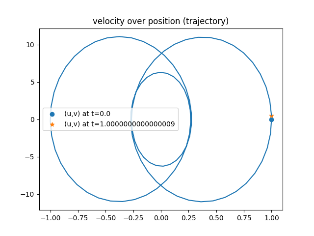
The solvers allow you to study the effect of different time stepping schemes on energy conservation. Newmark beta conserves energy:

Generalized alpha does not conserve energy:

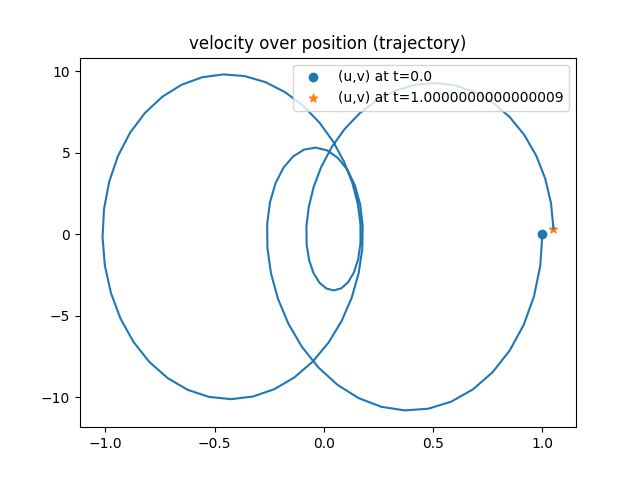
For details, refer to [1].

References

[1] V. Schüller, B. Rodenberg, B. Uekermann and H. Bungartz, A Simple Test Case for Convergence Order in Time and Energy Conservation of Black-Box Coupling Schemes, in: WCCM-APCOM2022. URL

[2] L. Willeke, D. Schneider and B. Uekermann, A preCICE-FMI Runner to Couple FMUs to PDE-Based Simulations, Proceedings 15th Intern. Modelica Conference, 2023. DOI