Multiple perpendicular flaps

Case Setup

In the following tutorial we model a fluid flowing through a channel. Two solid, elastic flaps are fixed to the floor of this channel. The flaps oscillate due to the fluid pressure building up on its surface. In this case, a fluid and two solids are coupled together using a fully-implicit multi-coupling scheme. The case setup is shown here:

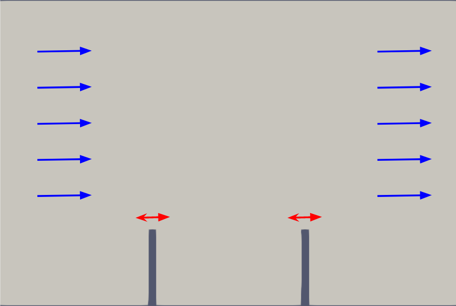
The simulated flow domain is 6 units long (x) and 4 units tall (z). The flaps are clamped at the bottom (z=0) and they are 1 unit tall (z), 0.1 units long (x), and 0.3 units wide (y). Being located at x=-1 and x=1, the flaps split the domain into three equal parts.

This is a quasi-2D simulation, with one cell in width and empty conditions are imposed on the front and back.

The inflow velocity is 5 m/s (uniform) on the left boundary. At the outlet, pressure is set to zero and velocity to zeroGradient. The top, bottom and flap are walls with a noslip condition.

For a case showing fluid-structure interaction only (no multi-coupling), take a look at the single perpendicular flap tutorial.

Configuration

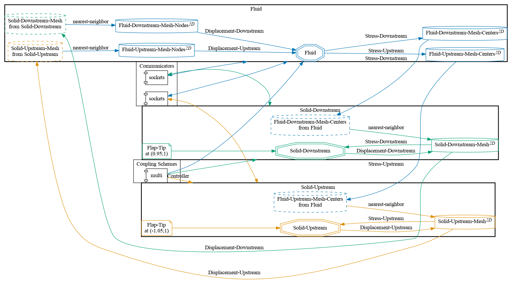
preCICE configuration (image generated using the precice-config-visualizer):

Why multi-coupling?

This is a case with three participants: the fluid and each flap. In preCICE, there are two options to couple more than two participants. The first option a composition of bi-coupling schemes, in which we must specify the exchange of data in a participant to participant manner. However, such a composition is not suited for combining multiple strong fluid-structure interactions [1]. Thus, in this case, we use the second option, fully-implicit multi-coupling.

We can set this in our precice-config.xml:

<coupling-scheme:multi>
  <participant name="Fluid" control="yes"/>
   <participant name="Solid-Upstream" />
   <participant name="Solid-Downstream" />

The participant that has the control is the one that it is connected to all other participants. This is why we have chosen the fluid participant for this task.

About the Solvers

For the fluid participant we use OpenFOAM. In particular, we use the application pimpleFoam. The geometry of the Fluid participant is defined in the file Fluid/system/blockMeshDict. Besides, we must specify where are we exchanging data with the other participants. The interfaces are set in the file Fluid/system/preciceDict. In this file, we set to exchange stress and displacement on the surface of each flap.

Most of the coupling details are specified in the file precice-config.xml. Here we estipulate the order in which we read/write data from one participant to another or how we map from the fluid to the solid’s mesh. In particular, we have chosen the nearest-neighbor mapping scheme.

For the simulation of the solid participants we use the deal.II adapter. In deal.II, the geometry of the domain is specified directly on the solver. The two flaps in our case are essentially the same but for the x-coordinate. The flap geometry is given to the solver when we select the scenario in the .prm file.

set Scenario            = PF

But to specify the position of the flap along the x-axis, we must specify it in the solid-upstream-dealii/parameters.prm file as follows:

set Flap location     = -1.0

While in case of solid-downstream-dealii/parameters.prm we write:

set Flap location     = 1.0

The scenario settings are implemented similarly for the nonlinear case.

Running the Simulation

1. Preparation: To run the coupled simulation, copy the deal.II executable elasticity into the main folder. To learn how to obtain the deal.II executable take a look at the description on the deal.II-adapter page.

2. Starting:

   We are going to run each solver in a different terminal. It is important that first we navigate to the simulation directory so that all solvers start in the same directory. To start the Fluid participant, run:

   cd fluid-openfoam
   ./run.sh
   

   to start OpenFOAM in serial or

   cd fluid-openfoam
   ./run.sh -parallel
   

   for a parallel run.

   The solid participants are only designed for serial runs. To run the Solid-Upstream participant, execute the corresponding deal.II binary file e.g. by:

   cd solid-upstream-dealii
   ./run.sh
   

   Finally, in the third terminal we will run the solver for the Solid-Downstream participant by:

   cd solid-downstream-dealii
   ./run.sh
   

Postprocessing

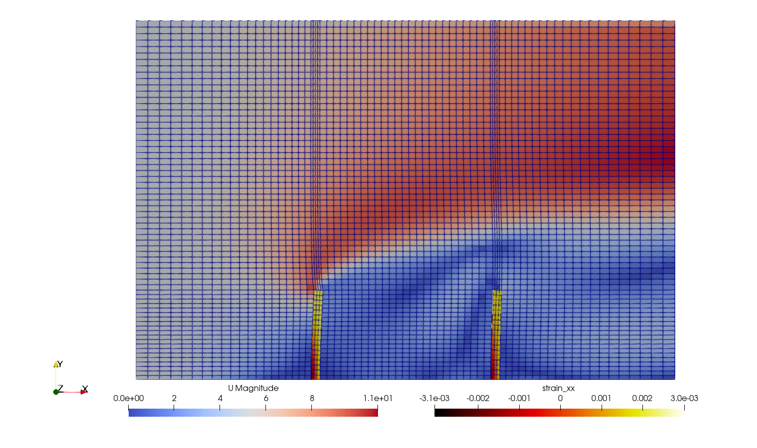
After the simulation has finished, you can visualize your results using e.g. ParaView. Fluid results are in the OpenFOAM format and you may load the fluid-openfoam.foam file. Looking at the fluid results is enough to obtain information about the behaviour of the flaps. You can also visualize the solid participants’ vtks though.

Example visualization of the fluid velocity and the solid displacement at t=2.3s, after synchronizing the results with a Temporal Shift Scale filter (scale for the deal.II results: 0.1):

References

[1] H. Bungartz, F. Linder, M. Mehl, B. Uekermann. A plug-and-play coupling approach for parallel multi-field simulations. Comput Mech 55, 1119-1129 (2015). https://doi.org/10.1007/s00466-014-1113-2