Setup
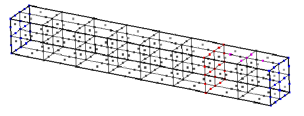
We have a rectangular linear elastic beam of dimensions 1 x 1 x 8 m, divided in two subdomains by a splitting plane at z = 6 m. This plane corresponds to the coupling surface. Both ends of the beam (z = 0 and z = 8 m) are fixed. A mechanical load F = -0.001 N is applied constantly along the y-axis onto a small set of nodes near the end of the beam. These boundary conditions can be seen in the input files beam<x>.inp. Initial conditions are zero both for position and velocity. Other parameters can be found and customized in the .inp files.

Configuration
preCICE configuration (image generated using the precice-config-visualizer):

Available solvers
- CalculiX. CalculiX is used for both structural parts. For more information, have a look at the CalculiX adapter documentation for more.
Running the Simulation
The prepared case already contains configuration and mesh files, so that the simulation is ready to run. You can start the simulation by running the script ./run.sh located in each participant directory. You will see both participants of the simulation running simultaneously.
Post-processing
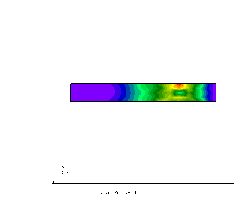
To see an animated visualization of the results, you can run the script ./visualize.py. It joins the *.frd output files of both participants to form a new file with the entire beam. Then, it calls cgx, since CalculiX results can only be visualized with this graphic tool. If you want to use e.g. ParaView, you may use converting tools.

You can open result files directly with cgx with the command cgx beam1.frd, for instance.