Perpendicular flap

Setup

We model a two-dimensional fluid flowing through a channel. A solid, elastic flap is fixed to the floor of this channel. The flap oscillates due to the fluid pressure building up on its surface. The setup is shown schematically here:

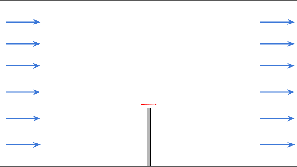
The simulated flow domain is 6 units long (x) and 4 units tall (y). The flap is located at the center of the bottom (x=0) and is 1 unit long (y) and 0.1 units thick (x). We set the fluid density \(\rho_F= 1.0kg/m^{3}\), the kinematic viscosity \(\nu_f= 1.0m^{2}/s\), the solid density \(\rho_s= 3.0·10^{3}kg/m^{3}\), the Young’s modulus to \(E= 4.0·10^{6} kg/ms^{2}\) and the Poisson ratio \(\nu_s = 0.3\). On the left boundary a constant inflow profile in x-direction of 10m/s is prescribed. The right boundary is an outflow and the top and bottom of the channel as well as the surface of the flap are no-slip walls.

Configuration

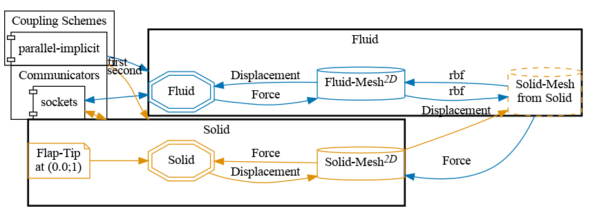
preCICE configuration (image generated using the precice-config-visualizer):

Available solvers

Fluid participant:

• OpenFOAM (pimpleFoam). In case you are using a very old OpenFOAM version, you will need to adjust the solver to pimpleDyMFoam in the Fluid/system/controlDict file. For more information, have a look at the OpenFOAM adapter documentation.

• SU2. As opposed to the other two fluid codes, SU2 is in particular specialized for compressible flow. Therefore the default simulation parameters haven been adjusted in order to pull the setup into the compressible flow regime. For more information, have a look at the SU2 adapter documentation.

• Nutils. For more information, have a look at the Nutils adapter documentation. This Nutils solver requires at least Nutils v6.0. This case currently takes orders of magnitude longer than the OpenFOAM and SU2 cases, see related issue.

• Fake. A simple python script that acts as a fake solver and provides an arbitrary force, linearly-increasing per length of the flap. This solver can be used for debugging of the solid participant and its adapter. It also technically works with implicit coupling, thus no changes to the preCICE configuration are necessary. Note that ASTE’s replay mode has a similar use case and could also feed artificial or previously recorded real data, replacing an actual solver.

Solid participant:

• FEniCS. The structural model is currently limited to linear elasticity. For more information, have a look at the FEniCS adapter documentation.

• CalculiX. In order to allow a reasonable comparison to all solid codes, the geometrically non-linear solver has been disabled and only a linear model is used by default. For more information, have a look at the CalculiX adapter documentation. Two cases are provided: one as a regular simulation, and one with modal dynamic simulations where a few eigenmodes are computed, and then used to simulate a reduced model. In that case, the run.sh script runs the frequency analysis, renames the output file to match with the actual input file, and then runs it. For more details, see the adapter configuration documentation. To run the modal dynamic version, add the -modal argument to the run.sh script.

• deal.II. This tutorial works only with Model = linear since the deal.II codes were developed with read data Stress instead of Force as applied here (example given in Turek-Hron-FSI) in the first place. The ./run.sh script takes the compiled executable elasticity as input argument (run.sh -e=/path/to/elasticity) and is required in case the executable is not discoverable at runtime (e.g. has been added to the system PATH). For more information, have a look at the deal.II adapter documentation.

• DUNE. For more information, have a look at the experimental DUNE adapter and send us your feedback.

• Nutils. The structural model is currently limited to linear elasticity. For more information, have a look at the Nutils adapter documentation. This Nutils solver requires at least Nutils v8.0.

• solids4foam. Like for CalculiX, the geometrically non-linear solver is used by default. For more information, see the solids4foam documentation and a related tutorial. This case works with solids4foam v2.0, which is compatible with up to OpenFOAM v2012 and OpenFOAM 9 (as well as foam-extend, with which the OpenFOAM-preCICE adapter is not compatible), as well as the OpenFOAM-preCICE adapter v1.2.0 or later.

• OpenFOAM (solidDisplacementFoam). For more information, have a look at the OpenFOAM plateHole tutorial. The solidDisplacementFoam solver only supports linear geometry and this case is only provided for quick testing purposes, leading to outlier results. For general solid mechanics procedures in OpenFOAM, see solids4foam.

Running the Simulation

All listed solvers can be used in order to run the simulation. OpenFOAM can be executed in parallel using run.sh -parallel. The default setting uses 4 MPI ranks. Open two separate terminals and start the desired fluid and solid participant by calling the respective run script run.sh located in the participant directory. For example:

cd fluid-openfoam
./run.sh

and

cd solid-fenics
./run.sh

in order to use OpenFOAM and FEniCS for this test case.

Post-processing

How to visualize the simulation results depends on the selected solvers. Most of the solvers generate vtk files which can visualized using, e.g., ParaView.

CalculiX exports results in .frd format, which you can visualize in CGX (cgx flap.frd). In the CGX window, you can click-and-hold to select different times and fields, or to animate the geometry. If you prefer to work with VTK files, you can also use tools such as ccx2paraview or a converter included in the calculix-adapter/tools directory.

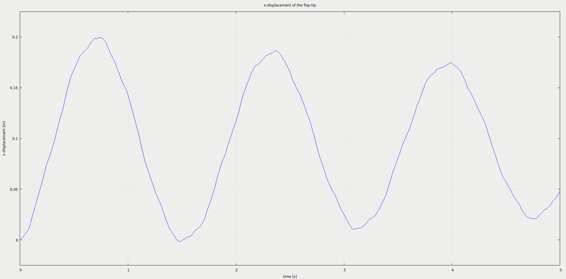
As we defined a watchpoint on the ‘Solid’ participant at the flap tip (see precice-config.xml), we can plot it with gnuplot using the script plot-displacement.sh. You need to specify the directory of the selected solid participant as a command line argument, so that the script can pick-up the desired watchpoint file, e.g. plot-displacement.sh solid-fenics. The resulting graph shows the x displacement of the flap tip. You can modify the script to plot the force instead.

There is moreover a script plot-all-displacements.sh to plot and compare all possible variants. This script expects all watchpoint logs to be available in a subfolder watchpoints in the format openfoam-dealii-version.log or similar. If you want to use this script, you need to edit it to exclude combinations you want to exclude and copy the files over accordingly.

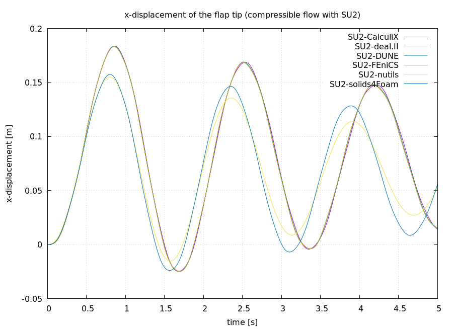
You should get results similar to this one:

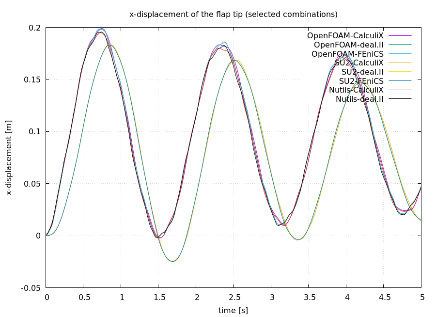
Reasons for the differences:

• The CalculiX adapter only supports linear finite elements (deal.II uses 4th order, FEniCS 2nd order).
• SU2 models a compressible fluid, OpenFOAM and Nutils an incompressible one.

Looking closer

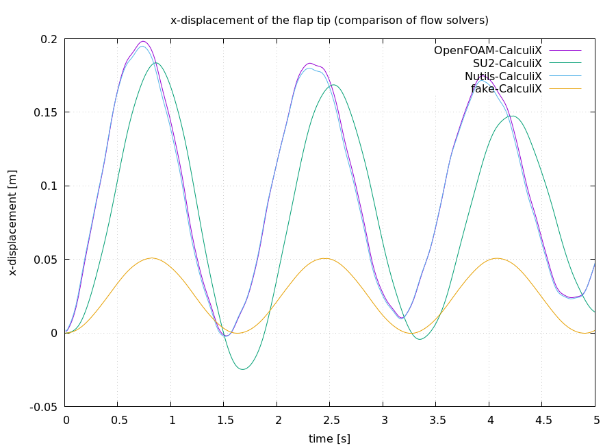
Excluding the solid-openfoam (outlier, provided mainly for technical testing), let’s look at an overview of different combinations.

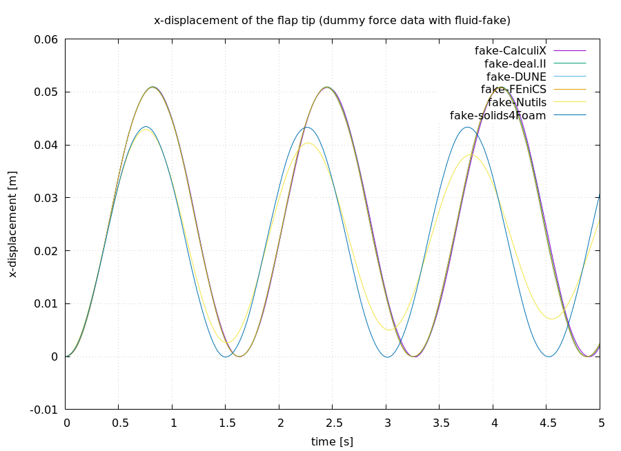
Comparison of the different flow solvers (incompressible fluid-openfoam and fluid-nutils, compressible fluid-su2, dummy fluid-fake):

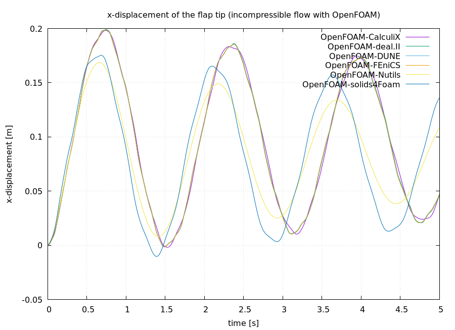
Combinations using the incompressible fluid-openfoam case:

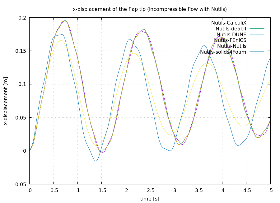
Combinations (excerpt) using the incompressible fluid-nutils case:

Combinations (excerpt) using the compressible fluid-su2 case:

Combinations (excerpt) using the dummy fluid-fake case: