Setup
The setup is exactly the same as described in our flow-over-heated-plate tutorial.
Available solvers
Fluid participant:
- OpenFOAM (buoyantPimpleFoam). For more information, have a look at the OpenFOAM adapter documentation.
Solid participant:
- OpenFOAM (laplacianFoam). For more information, have a look at the OpenFOAM adapter documentation.
The solvers are currently only OpenFOAM related. For information regarding the nearest-projection mapping, have a look in the OpenFOAM configuration section.
Configuration
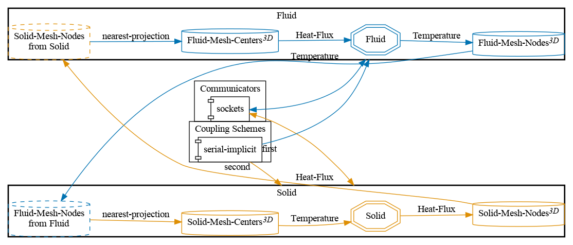
preCICE configuration (image generated using the precice-config-visualizer):
Running the Simulation
Open two separate terminals and start each participant by calling the respective run script.
cd fluid-openfoam
./run.sh
and
cd solid-openfoam
./run.sh
You can also run OpenFOAM in parallel by ./run.sh -parallel.
Changes in the Simulation Setup
As we are defining two meshes for each participant, we need to define them in the precice-config.xml and preciceDict configuration files. Additionally, we need to enable the connectivity switch for the adapter.
Changes in precice-config.xml
In order to map from face nodes to face centers, both meshes need to be specified. The nodes-based mesh uses the write data and the centers-based mesh uses the read data. Have a look in the given precice-config.xml in this tutorial. Example: Temperature is calculated by the Fluid participant and passed to the Solid participant. Therefore, it is the write data of the participant Fluid and the read data of the participant Solid. This results in the following two meshes for this data:
<mesh name="Fluid-Mesh-Nodes">
  <use-data name="Temperature"/>
</mesh>
<mesh name="Solid-Mesh-Centers">
  <use-data name="Temperature"/>
</mesh>
All further changes follow from this interface splitting. Have a look in the given config files for all details.
Notes on 2D Cases
From the preCICE point of view, the simulation here is in 3D, as opposed to the original 2D case, as is often the case with 3D solvers (such as OpenFOAM). In such cases, we recommend keeping the out-of-plane thickness of the domain small and comparable to the in-plane cell size. Otherwise, the face centers will have a large distance to the face nodes, which might trigger a preCICE warning and preCICE may even filter out one of the meshes, especially in parallel simulations.
Post-processing
Have a look at the flow-over heated-plate tutorial for the general aspects of post-processing.
Since we now defined mesh connectivity on our interface, we can export the coupling interface with the tag <export:vtk directory="precice-exports" /> in our precice-config.xml.
Visualizing these files (e.g. using ParaView) will show a triangular mesh, even though you use hexahedral meshes. This has nothing to do with your mesh and is just caused by the way the connectivity is defined in preCICE. As described above, the function setMeshTriangles is used to define the connectivity. Hence, every interface cell/face is represented by two triangles. The following image should give you an impression of a possible triangulated coupling mesh, which consists purely of hexahedral cells:
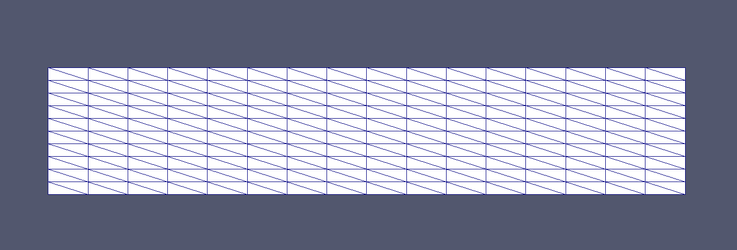
Connectivity is defined on meshes associated with mesh nodes, which are named respectively e.g. Fluid-Mesh-Nodes. In this case, you could directly see the interface without applying filters by loading the .vtk files. In order to visualize additionally center based meshes, where no connectivity is provided, select a Glyph filter in ParaView. Furthermore, it makes a difference, on which participant the <export... tag is defined in your precice-config.xml file. Each participant exports interface meshes, which he provides or receives. The receiving participant filters out mesh parts that it does not need (for the mapping). Hence, a received mesh might look incomplete.